Month: December 2018

Cleaning out: a 2011 Sankey goodie

As I am cleaning out my office – throwing away old notes, brochures and journals – I came across a November 2011 copy of German ‘UmweltMagazin (Environment Magazine). It has this Sankey diagram in an article on CO2-neutral steam generation for bioethanol production.


This Sankey diagram is in German. Flows are kW. This is for a small-scale plant at an agricultural business and heat is used for a destillation unit. The input feed to the steam boiler is primarily off-heat from a CHP plant fired with biomass. Losses are shown as grey arrows, steam as lilac arrows and heat in red. Condensate recovered at the heat excanger is fed back into the steam boiler (green loop).

Sorry for the quality of the scan. And Happy New Year to all of you! Will be back in 2019 with more Sankey diagrams.

Sankey Charts in Tableau

Found an interesting blog post over at TabVizExplorer, a casual blog maintained by Mithun Desai. Data visualization is one focus of his work.

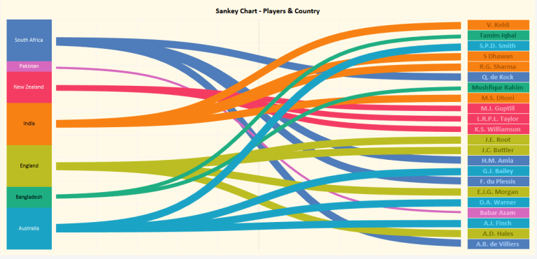
He uses Tableau to draw Sankey charts (I prefer to call them relationship diagrams, alluvial diagrams or even Spaghetti diagrams). Here is a rather simple one, showing the relation between top 20 cricket players and their country of origin.


The diagram has two data categories. The country of origin shown in the left stacked column in no particular order, and the top 20 players ordered according to their ICC ranking score.
In between are the streams or bands (or ‘Spaghettis’ for the sake of it) color coded by country of origin.

Now, it is not up to me criticizing the choice of diagram type for conveying this specific information. The author seems to have chosen the cricket topic just as a sample, to explain how to do Sankey charts in Tableau in general. Actually the colored list of top 20 (right column) already tells us all we need to know and you wouldn’t even need the left column and the streams.

The main reason I am not happy with this diagram is the fact that it does not stick to the most important characteristic of a Sankey diagram. The post itself comes with the definition: “Sankey diagrams are specific type of flow diagram in which the width of the arrows is shown proportionally to the flow quantity.”

So, what is the flow quantity here? I was thinking of net worth in $$$ of each player, or at least a translation of the ranking score to the width of the bands. But then Babar Azam, who ranked 4th with a score of 846 wouldn’t be shown with a band narrower than the one of E.J.G.Morgan coming in 20th with a score of 650. My guess is, that the the widths of the streams are chosen deliberately…

Where the bands merge, they overlap rather than merge to show the sum of the flow quantities. This makes for a very odd visual effect, at least in terms of Sankey diagrams.

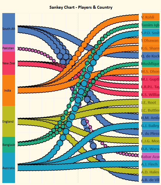
The blog article gives away some of the math behind the curves, so called Sigmoid curves, which is interesting.


This capture taken from the embedded Tableau graph shows how the curves are made up and how the width is maintained along the routing of each curve: You do it with cricket balls 😉 … or christmas bulbs.

Other implementations of relationship diagrams use Beziers curves (which sometimes come with another downside, read here). But that’s for another time…
LatAm BEN – Brazil

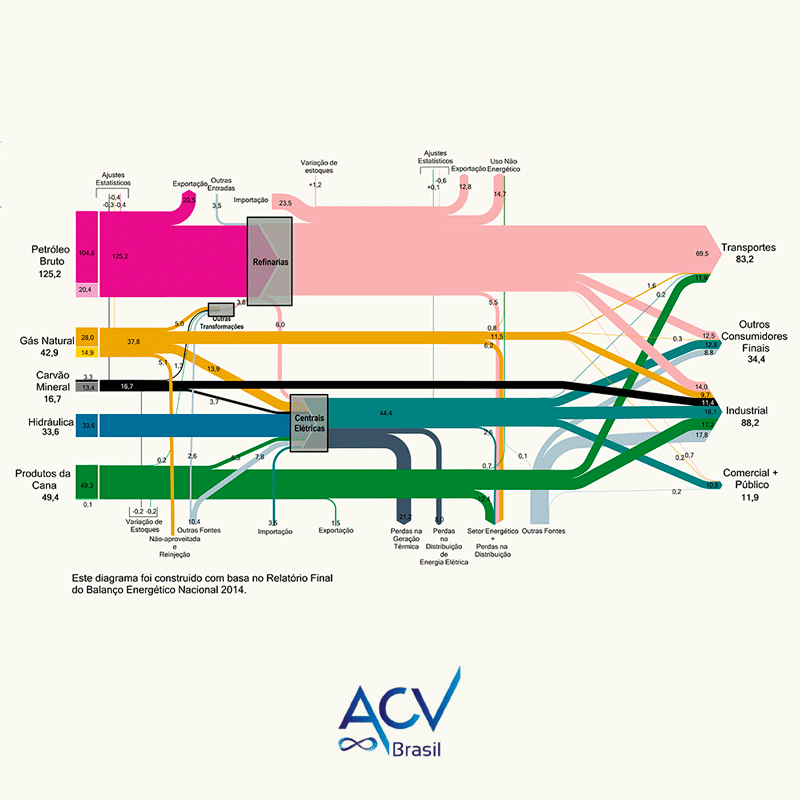
Working my way up the southern cone, here is the Balanço Energético Nacional 2014 for Brazil. Found this on the webpage of Curitiba based consulting firm ACV Brasil.

The national energy balances for Brazil are published annually by the Ministério de Minas e Energia (MME), and newer reports are available (PDF for 2018, large!). However, the energy flows diagrams in these official reports are less refined, so I opted to go with the remake by ACV.


The unit of flow is not shown, but my guess is that it is Mtep. like in the original publication.

Gudalquivir River Basin Water Flows

I discovered this Sankey diagram in an article by Gutiérrez-Martín, C.; Borrego-Marín, M.M.; Berbel, J. on ‘The Economic Analysis of Water Use in the Water Framework Directive Based on the System of Environmental-Economic Accounting for Water: A Case Study of the Guadalquivir River Basin” (published in Water 2017, 9, 180, open access article licensed under Creative Commons (CC BY 4.0). The Guadalquivir river basin is in Andalusia, Southern Spain.

The authors note that Sankey diagrams for water flows in a river basin or catchment area are useful because they show “at a glance, several aspects of the water cycle such as economic units, abstraction, supply, use, consumption, and returns to environment (soil water not included). In studying water use pathways, Sankey diagrams illustrate quantitative information about flows, their relationships, and their transformations.”

We see water taken (“abstracted”) from surface or groundwater by water supply companies and other users, distribution and water consumption by sectors, water flows ‘lost’ to the atmosphere and return of water to the environment.

Flows in this diagram are in hm³ (cubic hectometres). Note that they decided to use another scale for water used for energy generation (x 10 hm³) since otherwise the yellow-beige would be 10 times wider and maybe spoil the whole diagram.

The diagram has a top-down orientation and numerous loops and flow feedbacks, in contrast to the typical distribution diagrams (aka alluvial diagrams). It is well structured, nicely crafted and pleasing to the eye. Definitely on my top 10 list for 2018.

Global Agriculture Biomass Flows 2010

An interesting Sankey diagram on Global Biomass Flows 2010 can be found on the PBL Netherlands Environmental Assessment Agency website.


(Author: PBL, published under Creative Commons License CC BY 3.0)

This is from a research report ‘Integrated analysis of global biomass flows in search of the sustainable potential for bioenergy production’ published 2014 (available here) that estimates the worldwide biomass flows. It explains: “The biomass flows in the agro complex are presented in ExaJoules in the Sankey diagram (…). Using energy density data for all common commodities, the mass data have been converted to energy data. The energy content depends on the moisture content. In this study, the commonly referred weight–energy ratio’s were used.”

Basically, the diagram is made up from two main strands or pathways for biomass that are interlinked: In the top half the food production from agricultural soils (both crops and livestock breeding). In the lower half the grassland/meadows.

This is exclusively for the agricultural sector. The forestry sector is covered in a separate Sankey diagram (in one of my upcoming posts).

Note that small flow quantities (<3 EJ) are not to scale but rather have a minimum arrow width to keep them visible.